Coordinate Transformations
TerraScan can apply a coordinate transformation to point clouds at different steps of the processing workflow, for example, when loading or importing points, working with the points in RAM, processing points in batch mode in a TerraScan project or with a macro step, or writing points to output files. Coordinate transformations may also be applied to trajectories.
TerraScan divides coordinate transformations into several categories:
•Projection system transformations - used to transform coordinates from one coordinate system to another.
•User-defined transformations - coordinate transformations which can be defined by a number of parameters or equations.
•Geoid adjustment - used to transform elevation values from one height model to another.
•Systematic elevation or XY(Z) correction - applies a shift or rubbersheet correction to elevation values or an XY(Z) shift..
Projection system transformations
The transformation of coordinates from one coordinate system to another is a common task. Usually, the coordinates of raw laser data or trajectories are given in WGS84 or some UTM projections system values. For data processing and/or delivery, it is often necessary to transform these coordinates into another (national) projection system.
Coordinates in WGS84 system can be provided as longitude, latitude, ellipsoidal elevation values or geocentric XYZ values. TerraScan automatically recognizes the coordinate value format when it reads the points or trajectories.
The transformation into the destination coordinate system is usually done when point cloud data or trajectories are imported into TerraScan, for example, at the beginning of the processing workflow, or when data is prepared for delivery.
Projection systems are referenced by their EPSG code (EPSG = European Petroleum Survey Group Geodesy, worldwide unique 4- to 5-digits code numbers for coordinate systems). TerraScan implements a number of projection systems. A list of all available projection systems is provided in the Browse for Projection System dialog. If a projection system is not available in the EPSG code list, it can be defined in Coordinate transformations / User projection systems. All systems activated there are also available for a Projection change transformation.
There are different types of transformations that can be used to manipulate the coordinate values of point cloud data and trajectories in TerraScan. The implemented transformation types are:
•3D translate & rotate transformation
You can define the values for the transformation parameters in Coordinate transformations / Transformations category of TerraScan Settings.
The elevation values of raw laser data and trajectories are often provided as ellipsoidal height values. Usually, these values need to be transformed into orthometric values of a local height system.
For larger areas, the adjustment from ellipsoidal to orthometric height values can not be defined as one mathematical formula. Therefore, the elevation adjustment model needs to be defined by using local points for which the elevation difference between the height systems is known.
In TerraScan, the elevation adjustment can be performed for loaded points. See Adjust to geoid command for loaded points and Adjust to geoid command for trajectories for more information.
Elevation adjustment model
TerraScan implements a number of national, continental or global geoid models. The corresponding files are provided with the installation of a bundle package (Terrasolid installation bundle for Spatix or Microstation) and stored in the \GEOID folder of the Terra installation directory.
Alternatively, the input model for geoid adjustment may be provided in one of the following formats:
•Points from file - text file containing space-delimited X Y dZ- points.
•TerraModeler surface - triangulated surface model created from X Y dZ - points. The surface model in TerraModeler has the advantage that you can visualize the shape of the adjustment model.
•Selected linear chain - linear element of which the vertices represent the X Y dZ - points.
XY are the easting and northing coordinates of the geoid model points, dZ is the elevation difference between ellipsoidal and local heights at the location of each geoid model point. Intermediate adjustment values of the model are derived by aerial (text file or surface model as input) or linear (linear element as input) interpolation between the known geoid model points.
The figure below illustrates the aerial interpolation method. The yellow shape represents a project area covered by data, the red points symbolize known X Y dZ - points and the green points interpolated X Y dZ - points. The red (dotted) lines show the triangulated model.
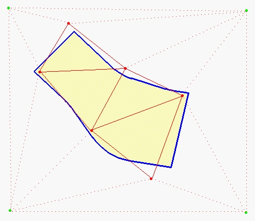
The six known points in the illustration above do not create a model that completely encloses the project area. If the model does not provide any additional information, TerraScan automatically adds four corner points (green points in the illustration) to expand the elevation adjustment model. Each added corner point has the same dz value as the closest known point.
It is recommended to use an adjustment model that exceeds the project area and thus, provides more accurate elevation information for project boundaries.
Systematic elevation or XY(Z) correction
A systematic correction needs to be applied if the point cloud data are systematically shifted in elevation and/or in XY. The systematic shift can be detected by comparing the point cloud with ground control points (GCPs).
TerraScan can do the comparison automatically. The GCPs must be provided in a text file which stores an identifier (optionally), X, Y and Z coordinates in space-delimited fields, one line for each control point. The identifier is normally a number but it may include non-numeric characters as well.
In the point cloud, at least the points on the ground around the GCP locations should be classified into a separate class. In practice, the check of a systematic elevation shift is often done after the ground points have been classified in the point cloud. The check of a systematic elevation shift can be performed for loaded points.
An XY(Z) correction can only be applied to loaded points. The check of an XY shift requires the definition of signal markers for GCP locations. The signal markers must be visible in the intensity display of the point cloud. Thus, signal markers must be drawn on the ground, preferable as white signal on a dark background, before the data is collected. Signal marker shapes can be defined in the Signal markers category of TerraScan Settings and then used in the Output control report command for loaded points. The proper use of signal markers requires a relatively high point density and is best suited for point clouds collected with a UAV-carried system.
To apply a systematic correction to a loaded point cloud, proceed as follows:
1. Create a control report using Output control report command for loaded points.
2. Check the correction values. If necessary, improve a signal marker position manually.
3. Apply the correction by using commands from the Apply pulldown menu of the Control report window.
You can type the dz value directly into the Transform loaded points dialog if you want to apply the elevation adjustment to loaded points only. In this case, you do not need to define a transformation in TerraScan Settings.
Control point report
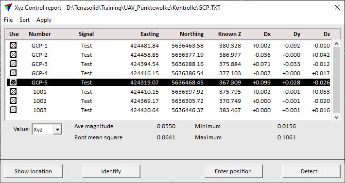
The control point report is shown in the Control report or Xyz Control report window:
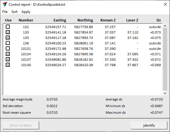
The window contains the list of all GCPs in the input text file. For each point, the following information is shown:
•Use - determines whether a GCP is used in the comparison or not. Switch control points on or off by clicking on the square.
•Number - identifier of the GCP.
•Signal - name of the signal marker used for a GCP. This is only shown if XYZ is checked.
•Easting - easting coordinate of the GCP.
•Northing - northing coordinate of the GCP.
•Known Z - elevation coordinate of the GCP.
•Laser Z - elevation value derived from the point cloud at the GCP’s XY location. This is only shown if elevation is checked.
•Dx - difference between the GCP’s easting value and the easting value derived from the signal marker. This is only shown if XYZ is checked.
•Dy - difference between the GCP’s northing value and the northing value derived from the signal marker. This is only shown if XYZ is checked.
•Dz - difference between Known Z and Laser Z. (Elevation check only) If the value exceeds a limit defined in the Control report settings, the value is displayed in red. If a control point is outside the area covered with point cloud data, the Dz value is shown as "outside".
•Intensity - weighted intensity value of the three closest laser points at the GCP’s XY location. A closer laser point influences the value more than a more distant laser point. This is displayed if the option in the Control report settings is switched on.
•Line - line number assigned to the laser points at the GCP’s XY location. This is displayed if the option in the Control report settings is switched on.
Below the GCP list, some statistical information computed from the difference values is provided. This includes average magnitude, standard deviation of a single value (X, Y or Z) and root mean square. Additionally, the average of single values, minimum and maximum value of differences is displayed. For XYZ check, you may select a value in the Value list for which you want to see the statistics.
The report can be saved into a text file or sent to a printer using Save as text or Print commands from the File pulldown menu.
The GCPs in the list can be sorted in different ways using the commands from the Sort pulldown menu.
For loaded points, you can apply the correction shown in the report window by using commands from the Apply pulldown menu.
If a line in the list is selected, the CAD file views defined in the Control report settings are centered at the location of the corresponding GCP.
To show the location of a GCP, select a line in the list. Click on the Show location button and move the mouse pointer into a view. This highlights the selected GCP with a square (elevation check) or with the shape of the signal marker (XYZ check).
To identify a GCP, click on the Identify button and place a data click close to a GCP in a view. This selects the corresponding line in the list.
If the software did not detect the XY location of a signal marker accurate enough, you can place the control point location manually by using the Enter position button or try the detection again by using the Detect button. A click on the button opens the Enter signal position or the Detect signal location dialog:
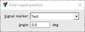
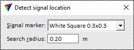
Define settings and place a data click at the location of the control point. In case of manual placement, the data click determines the XY location of the signal measurement. The automatic detection tries to identify the signal marker in the point cloud and derives the XY position.
SETTING |
EFFECT |
|---|---|
Signal marker |
Name of the signal marker as defined in the Signal markers category of TerraScan Settings. |
Angle |
Horizontal rotation angle of the signal marker. For manual placement, the (rotated) signal marker shape is displayed at mouse pointer location. |
Search radius |
Radial distance around the data click within which the software tries to detect the signal marker shape in the intensity values. For automatic detection, the circle representing the search area is displayed at mouse pointer location. |
Commands from the Apply pulldown menu can be used to apply a correction to the loaded point cloud. This includes either a shift correction in XYZ, XY or Z (elevation), or a rubbersheet correction. A rubbersheet correction is based on a correction model where each GCP defines a correction vector. Between the GCPs, correction values are interpolated. A rubbersheet correction forces all difference values between GCPs and point cloud to 0.0. The following figure illustrates the method:
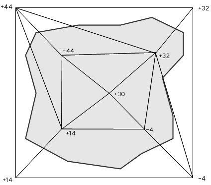
Numbers indicate, for example, elevation correction values.
To apply a systematic elevation shift or rubbersheet correction to loaded points:
1. Select Elevation shift command or Rubbersheet correction from the Apply pulldown menu.
A dialog is displayed which shows the shift value and asks for confirmation.
2. Confirm the correction by clicking Yes. Alternatively, you can can cancel the process by clicking No.
This applies the correction to the loaded point cloud. In the Control report window, the difference values and statistics are recomputed.
To apply a systematic XY(Z) shift correction to loaded points:
1. Select Shift command from the Apply pulldown menu.
This opens the Apply Shift dialog:
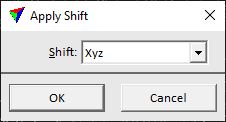
2. Select the dimension of the shift you want to apply and click OK.
This applies the systematic shift to the loaded point cloud. An information dialog shows the applied values. In the Xyz Control report window, the difference values and statistics are recomputed.
SETTING |
EFFECT |
|---|---|
Shift |
Dimension of the shift: •Xyz - systematic 3D correction in X, Y and Z. •Xy - systematic horizontal shift. •Z - systematic vertical shift. |
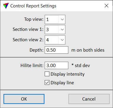
The display settings for the control point report can be changed using Settings command from the File pulldown menu. This opens the Control Report Settings dialog:
SETTING |
EFFECT |
|---|---|
Top view |
Top view that is updated if a GCP is selected. |
Section view 1 |
First section view that is updated if a GCP is selected. The section is drawn in east-west direction. |
Section view 2 |
Second section view that is updated if a GCP is selected. The section is drawn in north-east direction. |
Depth |
Depth of a section in the section views. The actual depth shown in a section view is the given value * 2. |
Hilite limit |
Determines the limit for displaying elevation difference values in red in the report. This is only available for elevation check. |
Display intensity |
If on, the average intensity value of the laser points at the GCP location is displayed in the report. This is only available for elevation check. |
Display line |
If on, the line number of the laser points at the GCP location is displayed in the report. This is only available for elevation check. |